
Classification with Python
In this notebook we try to practice all the classification algorithms that we learned in this course.
We load a dataset using Pandas library, and apply the following algorithms, and find the best one for this specific dataset by accuracy evaluation methods.
Lets first load required libraries:
import itertools
import numpy as np
import matplotlib.pyplot as plt
from matplotlib.ticker import NullFormatter
import pandas as pd
import numpy as np
import matplotlib.ticker as ticker
from sklearn import preprocessing
%matplotlib inline
About dataset
This dataset is about past loans. The Loan_train.csv data set includes details of 346 customers whose loan are already paid off or defaulted. It includes following fields:
| Field | Description |
|---|---|
| Loan_status | Whether a loan is paid off on in collection |
| Principal | Basic principal loan amount at the |
| Terms | Origination terms which can be weekly (7 days), biweekly, and monthly payoff schedule |
| Effective_date | When the loan got originated and took effects |
| Due_date | Since it’s one-time payoff schedule, each loan has one single due date |
| Age | Age of applicant |
| Education | Education of applicant |
| Gender | The gender of applicant |
Lets download the dataset
!wget -O loan_train.csv https://s3-api.us-geo.objectstorage.softlayer.net/cf-courses-data/CognitiveClass/ML0101ENv3/labs/loan_train.csv
--2019-03-12 10:06:53--  https://s3-api.us-geo.objectstorage.softlayer.net/cf-courses-data/CognitiveClass/ML0101ENv3/labs/loan_train.csv
Resolving s3-api.us-geo.objectstorage.softlayer.net (s3-api.us-geo.objectstorage.softlayer.net)... 67.228.254.193
Connecting to s3-api.us-geo.objectstorage.softlayer.net (s3-api.us-geo.objectstorage.softlayer.net)|67.228.254.193|:443... connected.
HTTP request sent, awaiting response... 200 OK
Length: 23101 (23K) [text/csv]
Saving to: ‘loan_train.csv’

100%[======================================>] 23,101      --.-K/s   in 0.002s

2019-03-12 10:06:53 (11.4 MB/s) - ‘loan_train.csv’ saved [23101/23101]
Load Data From CSV File
df = pd.read_csv('loan_train.csv')
df.head()
| Unnamed: 0 | Unnamed: 0.1 | loan_status | Principal | terms | effective_date | due_date | age | education | Gender | |
|---|---|---|---|---|---|---|---|---|---|---|
| 0 | 0 | 0 | PAIDOFF | 1000 | 30 | 9/8/2016 | 10/7/2016 | 45 | High School or Below | male |
| 1 | 2 | 2 | PAIDOFF | 1000 | 30 | 9/8/2016 | 10/7/2016 | 33 | Bechalor | female |
| 2 | 3 | 3 | PAIDOFF | 1000 | 15 | 9/8/2016 | 9/22/2016 | 27 | college | male |
| 3 | 4 | 4 | PAIDOFF | 1000 | 30 | 9/9/2016 | 10/8/2016 | 28 | college | female |
| 4 | 6 | 6 | PAIDOFF | 1000 | 30 | 9/9/2016 | 10/8/2016 | 29 | college | male |
df.shape
(346, 10)
Convert to date time object
df['due_date'] = pd.to_datetime(df['due_date'])
df['effective_date'] = pd.to_datetime(df['effective_date'])
df.head()
| Unnamed: 0 | Unnamed: 0.1 | loan_status | Principal | terms | effective_date | due_date | age | education | Gender | |
|---|---|---|---|---|---|---|---|---|---|---|
| 0 | 0 | 0 | PAIDOFF | 1000 | 30 | 2016-09-08 | 2016-10-07 | 45 | High School or Below | male |
| 1 | 2 | 2 | PAIDOFF | 1000 | 30 | 2016-09-08 | 2016-10-07 | 33 | Bechalor | female |
| 2 | 3 | 3 | PAIDOFF | 1000 | 15 | 2016-09-08 | 2016-09-22 | 27 | college | male |
| 3 | 4 | 4 | PAIDOFF | 1000 | 30 | 2016-09-09 | 2016-10-08 | 28 | college | female |
| 4 | 6 | 6 | PAIDOFF | 1000 | 30 | 2016-09-09 | 2016-10-08 | 29 | college | male |
Data visualization and pre-processing
Let’s see how many of each class is in our data set
df['loan_status'].value_counts()
PAIDOFF       260
COLLECTION     86
Name: loan_status, dtype: int64
260 people have paid off the loan on time while 86 have gone into collection
Lets plot some columns to underestand data better:
# notice: installing seaborn might takes a few minutes
!conda install -c anaconda seaborn -y
Fetching package metadata .............
Solving package specifications: .

Package plan for installation in environment /opt/conda/envs/DSX-Python35:

The following packages will be UPDATED:

    seaborn: 0.8.0-py35h15a2772_0 --> 0.9.0-py35_0 anaconda

seaborn-0.9.0- 100% |################################| Time: 0:00:00  47.36 MB/s
import seaborn as sns
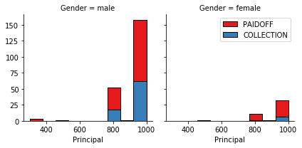
bins = np.linspace(df.Principal.min(), df.Principal.max(), 10)
g = sns.FacetGrid(df, col="Gender", hue="loan_status", palette="Set1", col_wrap=2)
g.map(plt.hist, 'Principal', bins=bins, ec="k")
g.axes[-1].legend()
plt.show()
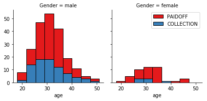
bins = np.linspace(df.age.min(), df.age.max(), 10)
g = sns.FacetGrid(df, col="Gender", hue="loan_status", palette="Set1", col_wrap=2)
g.map(plt.hist, 'age', bins=bins, ec="k")

g.axes[-1].legend()
plt.show()
Pre-processing: Feature selection/extraction
Lets look at the day of the week people get the loan
df['dayofweek'] = df['effective_date'].dt.dayofweek
bins = np.linspace(df.dayofweek.min(), df.dayofweek.max(), 10)
g = sns.FacetGrid(df, col="Gender", hue="loan_status", palette="Set1", col_wrap=2)
g.map(plt.hist, 'dayofweek', bins=bins, ec="k")
g.axes[-1].legend()
plt.show()
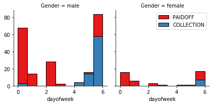
We see that people who get the loan at the end of the week dont pay it off, so lets use Feature binarization to set a threshold values less then day 4
df['weekend'] = df['dayofweek'].apply(lambda x: 1 if (x>3)  else 0)
df.head()
| Unnamed: 0 | Unnamed: 0.1 | loan_status | Principal | terms | effective_date | due_date | age | education | Gender | dayofweek | weekend | |
|---|---|---|---|---|---|---|---|---|---|---|---|---|
| 0 | 0 | 0 | PAIDOFF | 1000 | 30 | 2016-09-08 | 2016-10-07 | 45 | High School or Below | male | 3 | 0 |
| 1 | 2 | 2 | PAIDOFF | 1000 | 30 | 2016-09-08 | 2016-10-07 | 33 | Bechalor | female | 3 | 0 |
| 2 | 3 | 3 | PAIDOFF | 1000 | 15 | 2016-09-08 | 2016-09-22 | 27 | college | male | 3 | 0 |
| 3 | 4 | 4 | PAIDOFF | 1000 | 30 | 2016-09-09 | 2016-10-08 | 28 | college | female | 4 | 1 |
| 4 | 6 | 6 | PAIDOFF | 1000 | 30 | 2016-09-09 | 2016-10-08 | 29 | college | male | 4 | 1 |
Convert Categorical features to numerical values
Lets look at gender:
df.groupby(['Gender'])['loan_status'].value_counts(normalize=True)
Gender  loan_status
female  PAIDOFF        0.865385
        COLLECTION     0.134615
male    PAIDOFF        0.731293
        COLLECTION     0.268707
Name: loan_status, dtype: float64
86 % of female pay there loans while only 73 % of males pay there loan
Lets convert male to 0 and female to 1:
df['Gender'].replace(to_replace=['male','female'], value=[0,1],inplace=True)
df.head()
| Unnamed: 0 | Unnamed: 0.1 | loan_status | Principal | terms | effective_date | due_date | age | education | Gender | dayofweek | weekend | |
|---|---|---|---|---|---|---|---|---|---|---|---|---|
| 0 | 0 | 0 | PAIDOFF | 1000 | 30 | 2016-09-08 | 2016-10-07 | 45 | High School or Below | 0 | 3 | 0 |
| 1 | 2 | 2 | PAIDOFF | 1000 | 30 | 2016-09-08 | 2016-10-07 | 33 | Bechalor | 1 | 3 | 0 |
| 2 | 3 | 3 | PAIDOFF | 1000 | 15 | 2016-09-08 | 2016-09-22 | 27 | college | 0 | 3 | 0 |
| 3 | 4 | 4 | PAIDOFF | 1000 | 30 | 2016-09-09 | 2016-10-08 | 28 | college | 1 | 4 | 1 |
| 4 | 6 | 6 | PAIDOFF | 1000 | 30 | 2016-09-09 | 2016-10-08 | 29 | college | 0 | 4 | 1 |
One Hot Encoding
How about education?
df.groupby(['education'])['loan_status'].value_counts(normalize=True)
education             loan_status
Bechalor              PAIDOFF        0.750000
                      COLLECTION     0.250000
High School or Below  PAIDOFF        0.741722
                      COLLECTION     0.258278
Master or Above       COLLECTION     0.500000
                      PAIDOFF        0.500000
college               PAIDOFF        0.765101
                      COLLECTION     0.234899
Name: loan_status, dtype: float64
Feature befor One Hot Encoding
df[['Principal','terms','age','Gender','education']].head()
| Principal | terms | age | Gender | education | |
|---|---|---|---|---|---|
| 0 | 1000 | 30 | 45 | 0 | High School or Below |
| 1 | 1000 | 30 | 33 | 1 | Bechalor |
| 2 | 1000 | 15 | 27 | 0 | college |
| 3 | 1000 | 30 | 28 | 1 | college |
| 4 | 1000 | 30 | 29 | 0 | college |
Use one hot encoding technique to conver categorical varables to binary variables and append them to the feature Data Frame
Feature = df[['Principal','terms','age','Gender','weekend']]
Feature = pd.concat([Feature,pd.get_dummies(df['education'])], axis=1)
Feature.drop(['Master or Above'], axis = 1,inplace=True)
Feature.head()
| Principal | terms | age | Gender | weekend | Bechalor | High School or Below | college | |
|---|---|---|---|---|---|---|---|---|
| 0 | 1000 | 30 | 45 | 0 | 0 | 0 | 1 | 0 |
| 1 | 1000 | 30 | 33 | 1 | 0 | 1 | 0 | 0 |
| 2 | 1000 | 15 | 27 | 0 | 0 | 0 | 0 | 1 |
| 3 | 1000 | 30 | 28 | 1 | 1 | 0 | 0 | 1 |
| 4 | 1000 | 30 | 29 | 0 | 1 | 0 | 0 | 1 |
Feature selection
Lets defind feature sets, X:
X = Feature
X[0:5]
| Principal | terms | age | Gender | weekend | Bechalor | High School or Below | college | |
|---|---|---|---|---|---|---|---|---|
| 0 | 1000 | 30 | 45 | 0 | 0 | 0 | 1 | 0 |
| 1 | 1000 | 30 | 33 | 1 | 0 | 1 | 0 | 0 |
| 2 | 1000 | 15 | 27 | 0 | 0 | 0 | 0 | 1 |
| 3 | 1000 | 30 | 28 | 1 | 1 | 0 | 0 | 1 |
| 4 | 1000 | 30 | 29 | 0 | 1 | 0 | 0 | 1 |
What are our lables?
y = df['loan_status'].values
y[0:5]
array(['PAIDOFF', 'PAIDOFF', 'PAIDOFF', 'PAIDOFF', 'PAIDOFF'], dtype=object)
Normalize Data
Data Standardization give data zero mean and unit variance (technically should be done after train test split )
X= preprocessing.StandardScaler().fit(X).transform(X)
X[0:5]
array([[ 0.51578458,  0.92071769,  2.33152555, -0.42056004, -1.20577805,
        -0.38170062,  1.13639374, -0.86968108],
       [ 0.51578458,  0.92071769,  0.34170148,  2.37778177, -1.20577805,
         2.61985426, -0.87997669, -0.86968108],
       [ 0.51578458, -0.95911111, -0.65321055, -0.42056004, -1.20577805,
        -0.38170062, -0.87997669,  1.14984679],
       [ 0.51578458,  0.92071769, -0.48739188,  2.37778177,  0.82934003,
        -0.38170062, -0.87997669,  1.14984679],
       [ 0.51578458,  0.92071769, -0.3215732 , -0.42056004,  0.82934003,
        -0.38170062, -0.87997669,  1.14984679]])
Classification
Now, it is your turn, use the training set to build an accurate model. Then use the test set to report the accuracy of the model You should use the following algorithm:
- K Nearest Neighbor(KNN)
- Decision Tree
- Support Vector Machine
- Logistic Regression
__ Notice:__
- You can go above and change the pre-processing, feature selection, feature-extraction, and so on, to make a better model.
- You should use either scikit-learn, Scipy or Numpy libraries for developing the classification algorithms.
- You should include the code of the algorithm in the following cells.
K Nearest Neighbor(KNN)
Notice: You should find the best k to build the model with the best accuracy.
warning: You should not use the loan_test.csv for finding the best k, however, you can split your train_loan.csv into train and test to find the best k.
from sklearn.neighbors import KNeighborsClassifier
k = 6
#Train Model and Predict
model_knn = KNeighborsClassifier(n_neighbors = k)
model_knn.fit(X,y)
model_knn
KNeighborsClassifier(algorithm='auto', leaf_size=30, metric='minkowski',
           metric_params=None, n_jobs=1, n_neighbors=6, p=2,
           weights='uniform')
Decision Tree
from sklearn.tree import DecisionTreeClassifier
model_tree = DecisionTreeClassifier(criterion="entropy", max_depth = 4)
model_tree.fit(X,y)
model_tree # it shows the default parameters
DecisionTreeClassifier(class_weight=None, criterion='entropy', max_depth=4,
            max_features=None, max_leaf_nodes=None,
            min_impurity_decrease=0.0, min_impurity_split=None,
            min_samples_leaf=1, min_samples_split=2,
            min_weight_fraction_leaf=0.0, presort=False, random_state=None,
            splitter='best')
Support Vector Machine
from sklearn import svm
model_svm = svm.SVC(kernel='linear')
model_svm.fit(X, y)
model_svm
SVC(C=1.0, cache_size=200, class_weight=None, coef0=0.0,
  decision_function_shape='ovr', degree=3, gamma='auto', kernel='linear',
  max_iter=-1, probability=False, random_state=None, shrinking=True,
  tol=0.001, verbose=False)
Logistic Regression
from sklearn.linear_model import LogisticRegression
model_lr = LogisticRegression(C=0.0001, solver='liblinear')
model_lr.fit(X,y)
model_lr
LogisticRegression(C=0.0001, class_weight=None, dual=False,
          fit_intercept=True, intercept_scaling=1, max_iter=100,
          multi_class='ovr', n_jobs=1, penalty='l2', random_state=None,
          solver='liblinear', tol=0.0001, verbose=0, warm_start=False)
Model Evaluation using Test set
from sklearn.metrics import jaccard_similarity_score
from sklearn.metrics import f1_score
from sklearn.metrics import log_loss
First, download and load the test set:
!wget -O loan_test.csv https://s3-api.us-geo.objectstorage.softlayer.net/cf-courses-data/CognitiveClass/ML0101ENv3/labs/loan_test.csv
--2019-03-12 11:19:01--  https://s3-api.us-geo.objectstorage.softlayer.net/cf-courses-data/CognitiveClass/ML0101ENv3/labs/loan_test.csv
Resolving s3-api.us-geo.objectstorage.softlayer.net (s3-api.us-geo.objectstorage.softlayer.net)... 67.228.254.193
Connecting to s3-api.us-geo.objectstorage.softlayer.net (s3-api.us-geo.objectstorage.softlayer.net)|67.228.254.193|:443... connected.
HTTP request sent, awaiting response... 200 OK
Length: 3642 (3.6K) [text/csv]
Saving to: ‘loan_test.csv’

100%[======================================>] 3,642       --.-K/s   in 0s

2019-03-12 11:19:01 (680 MB/s) - ‘loan_test.csv’ saved [3642/3642]
Load Test set for evaluation
test_df = pd.read_csv('loan_test.csv')
test_df.head()
| Unnamed: 0 | Unnamed: 0.1 | loan_status | Principal | terms | effective_date | due_date | age | education | Gender | |
|---|---|---|---|---|---|---|---|---|---|---|
| 0 | 1 | 1 | PAIDOFF | 1000 | 30 | 9/8/2016 | 10/7/2016 | 50 | Bechalor | female |
| 1 | 5 | 5 | PAIDOFF | 300 | 7 | 9/9/2016 | 9/15/2016 | 35 | Master or Above | male |
| 2 | 21 | 21 | PAIDOFF | 1000 | 30 | 9/10/2016 | 10/9/2016 | 43 | High School or Below | female |
| 3 | 24 | 24 | PAIDOFF | 1000 | 30 | 9/10/2016 | 10/9/2016 | 26 | college | male |
| 4 | 35 | 35 | PAIDOFF | 800 | 15 | 9/11/2016 | 9/25/2016 | 29 | Bechalor | male |
# Prepare test set the same way the train set was evaluated
test_df['due_date'] = pd.to_datetime(test_df['due_date'])
test_df['effective_date'] = pd.to_datetime(test_df['effective_date'])
test_df['dayofweek'] = test_df['effective_date'].dt.dayofweek
test_df['weekend'] = test_df['dayofweek'].apply(lambda x: 1 if (x>3)  else 0)
test_df['Gender'].replace(to_replace=['male','female'], value=[0,1],inplace=True)

test_df[['Principal','terms','age','Gender','education']].head()
| Principal | terms | age | Gender | education | |
|---|---|---|---|---|---|
| 0 | 1000 | 30 | 50 | 1 | Bechalor |
| 1 | 300 | 7 | 35 | 0 | Master or Above |
| 2 | 1000 | 30 | 43 | 1 | High School or Below |
| 3 | 1000 | 30 | 26 | 0 | college |
| 4 | 800 | 15 | 29 | 0 | Bechalor |
Feature_test = test_df[['Principal','terms','age','Gender','weekend']]
Feature_test = pd.concat([Feature_test,pd.get_dummies(test_df['education'])], axis=1)
Feature_test.drop(['Master or Above'], axis = 1,inplace=True)
Feature_test.head()
| Principal | terms | age | Gender | weekend | Bechalor | High School or Below | college | |
|---|---|---|---|---|---|---|---|---|
| 0 | 1000 | 30 | 50 | 1 | 0 | 1 | 0 | 0 |
| 1 | 300 | 7 | 35 | 0 | 1 | 0 | 0 | 0 |
| 2 | 1000 | 30 | 43 | 1 | 1 | 0 | 1 | 0 |
| 3 | 1000 | 30 | 26 | 0 | 1 | 0 | 0 | 1 |
| 4 | 800 | 15 | 29 | 0 | 1 | 1 | 0 | 0 |
# Test data input
X_test = Feature_test
X_test = preprocessing.StandardScaler().fit(X_test).transform(X_test)
X_test[0:5]
# Test data output
from sklearn import metrics
y_test = test_df['loan_status'].values
y_test[0:5]
array(['PAIDOFF', 'PAIDOFF', 'PAIDOFF', 'PAIDOFF', 'PAIDOFF'], dtype=object)
# ACCURACY SCORES

# knn
yhat = model_knn.predict(X_test)
yhat
print("Train set KNN Accuracy: ", metrics.accuracy_score(y, model_knn.predict(X)))
print("Test set KNN Accuracy: ", metrics.accuracy_score(y_test, yhat))
knn_jaccard = jaccard_similarity_score(y_test, yhat)
knn_f1_score = f1_score(y_test, yhat, average='weighted')

# Decission tree
yhat = model_tree.predict(X_test)
yhat
print("Train set Decission Tree Accuracy: ", metrics.accuracy_score(y, model_tree.predict(X)))
print("Test set Decission Tree Accuracy: ", metrics.accuracy_score(y_test, yhat))
tree_jaccard = jaccard_similarity_score(y_test, yhat)
tree_f1_score = f1_score(y_test, yhat, average='weighted')

# SVM
yhat = model_svm.predict(X_test)
yhat
print("Train set SVM Accuracy: ", metrics.accuracy_score(y, model_svm.predict(X)))
print("Test set SVM Accuracy: ", metrics.accuracy_score(y_test, yhat))
svm_jaccard = jaccard_similarity_score(y_test, yhat)
svm_f1_score = f1_score(y_test, yhat, average='weighted')

# Logistic regression
yhat = model_lr.predict(X_test)
yhat_proba = model_lr.predict_proba(X_test)
yhat
print("Train set Logistic regression Accuracy: ", metrics.accuracy_score(y, model_lr.predict(X)))
print("Test set Logistic regression Accuracy: ", metrics.accuracy_score(y_test, yhat))
lr_jaccard = jaccard_similarity_score(y_test, yhat)
lr_f1_score = f1_score(y_test, yhat, average='weighted')
lr_log_loss = log_loss(y_test, yhat_proba)
Train set KNN Accuracy:  0.806358381503
Test set KNN Accuracy:  0.685185185185
Train set Decission Tree Accuracy:  0.751445086705
Test set Decission Tree Accuracy:  0.777777777778
Train set SVM Accuracy:  0.751445086705
Test set SVM Accuracy:  0.740740740741
Train set Logistic regression Accuracy:  0.745664739884
Test set Logistic regression Accuracy:  0.759259259259


/opt/conda/envs/DSX-Python35/lib/python3.5/site-packages/sklearn/metrics/classification.py:1135: UndefinedMetricWarning: F-score is ill-defined and being set to 0.0 in labels with no predicted samples.
  'precision', 'predicted', average, warn_for)
report = pd.DataFrame(data=np.array([["KNN", knn_jaccard, knn_f1_score, np.nan],
                                     ["Decision Tree", tree_jaccard, tree_f1_score, np.nan],
                                    ["SVM", svm_jaccard, svm_f1_score, np.nan],
                                    ["LogisticRegression", lr_jaccard, lr_f1_score, lr_log_loss]]), columns=["Algorithm", "Jaccard", "F1-score", "LogLoss"])
report = report.set_index(["Algorithm", "Jaccard", "F1-score", "LogLoss"])
# Jaccard
report
| Algorithm | Jaccard | F1-score | LogLoss |
|---|---|---|---|
| KNN | 0.685185185185 | 0.681298582533 | nan |
| Decision Tree | 0.777777777778 | 0.728395061728 | nan |
| SVM | 0.740740740741 | 0.630417651694 | nan |
| LogisticRegression | 0.759259259259 | 0.671764237356 | 0.689904024181 |
Want to learn more?
IBM SPSS Modeler is a comprehensive analytics platform that has many machine learning algorithms. It has been designed to bring predictive intelligence to decisions made by individuals, by groups, by systems – by your enterprise as a whole. A free trial is available through this course, available here: SPSS Modeler
Also, you can use Watson Studio to run these notebooks faster with bigger datasets. Watson Studio is IBM’s leading cloud solution for data scientists, built by data scientists. With Jupyter notebooks, RStudio, Apache Spark and popular libraries pre-packaged in the cloud, Watson Studio enables data scientists to collaborate on their projects without having to install anything. Join the fast-growing community of Watson Studio users today with a free account at Watson Studio
Thanks for completing this lesson!
Author: Saeed Aghabozorgi
Saeed Aghabozorgi, PhD is a Data Scientist in IBM with a track record of developing enterprise level applications that substantially increases clients’ ability to turn data into actionable knowledge. He is a researcher in data mining field and expert in developing advanced analytic methods like machine learning and statistical modelling on large datasets.
Copyright © 2018 Cognitive Class. This notebook and its source code are released under the terms of the MIT License.